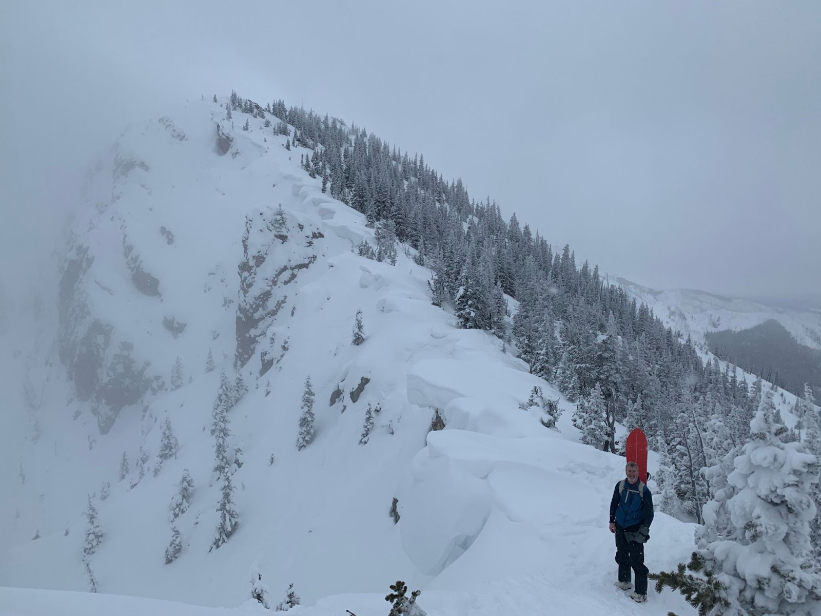
Slope Angle—Are You In the Danger Zone?

You have your beacon, shovel, probe, and maybe even an avalanche airbag, but what are you using for route planning and terrain assessment? If you’re new to digital maps and curious about the tools this technology can unlock, read on. 

Slope Angle is a critical component when assessing avalanche danger. It is defined as the angle a slope makes with the horizon, where completely flat is 0 degrees and vertical is 90 degrees. Slab avalanches occur most frequently on slopes between 30 and 45 degrees from horizontal. Anything above 45 degrees is generally too steep for a slab to form and anything less than around 30 degrees is too flat for a slab to slide. Knowing how to navigate in this danger zone can help us travel safer in the backcountry. Thanks to the NASA-funded Shuttle Radar Topography Mission (SRTM), we now have the data we need to calculate and visualize avalanche danger zones (based on slope angle) on a digitized map, anywhere on the planet.

In the past, we’ve relied on inclinometers—an in-field measurement to assess slope angle. While this type of measurement is an absolute must when traveling in the backcountry, a digitized slope angle layer can help with route planning both before a trip and in the field. In the onX Backcountry and Offroad apps, we display slope angle as a color-coded overlay that you can take with you, even when you don’t have an internet connection. 

Where Does Slope Angle Data Come From?

Slope angles, and most terrain analyses, rely on Digital Elevation Models (DEMs) which are digital representations of the height of the earth’s surface at any given location. There are two parameters we consider when using DEMs—spatial resolution and vertical accuracy. Spatial resolution is the area covered by a measurement. For example, a 30 meter spatial resolution means that a measurement of the height at a given point covers a 30 meter by 30 meter square on the ground. Vertical accuracy refers to the accuracy of the height measurement at that location. The 3D Elevation Program (3DEP) claims a vertical accuracy of 3.04 meters (95% confidence level) for the conterminous United States. There are two common techniques used to obtain this data: interferometry and Light Detection and Ranging (LIDAR). Interferometry is a method that relies on interference of radio, light, or UV waves to measure displacement, while LIDAR relies on differences in the time it takes a beam of coherent light (laser) to bounce off a surface. LIDAR-derived elevation data are typically higher resolution and more accurate than interferometric elevation data, with both vertical accuracy and horizontal resolutions below 3 meters. RADAR instruments on satellites hundreds of kilometers above the earth’s surface provide the source data for interferometric elevation, while LIDAR data is typically collected via fixed-wing aircraft. At onX, we’ve sourced high resolution terrain data, giving us a resolution for the U.S. in the range of 3 to 10 meters (and 25 meters for most of Canada) [3DEP, ArcticDEM, CDEM, and SRTM]. 

We provide slope angle data for four different horizontal resolutions or “zoom levels” [slippy map tile resolutions]: 11, 12, 13 and 14. Horizontal resolution refers to the number of measurements taken per meter along the surface of the earth. At each of these zoom levels a sample point (where a height measurement was recorded) represents a different horizontal distance. At zoom level 11, for example, a single measurement (one pixel) covers an area of 76 meters by 76 meters. As we zoom in (get closer to earth) we pass through each of the above zoom levels dividing the square’s side by 2. At level 12 our horizontal distance (one pixel) becomes 38 meters by 38 meters, while zoom level 14 gives us a pixel size of 9.6 meters by 9.6 meters. It is important to note that our vertical resolution remains constant (between 3 and 10 meters).

Takeaway: Zoom level 14 corresponds to a distance of about 9.6 meters, the slope angle at any point is the average slope covering an area measuring 9.6 meters by 9.6 meters. In our field testing, we found this resolution provided the right amount of information to aid in terrain assessment without overwhelming map download sizes; and yes, you can and should take this data offline. 

Let’s Define Slope Angle

Consider a simple two-dimensional line:

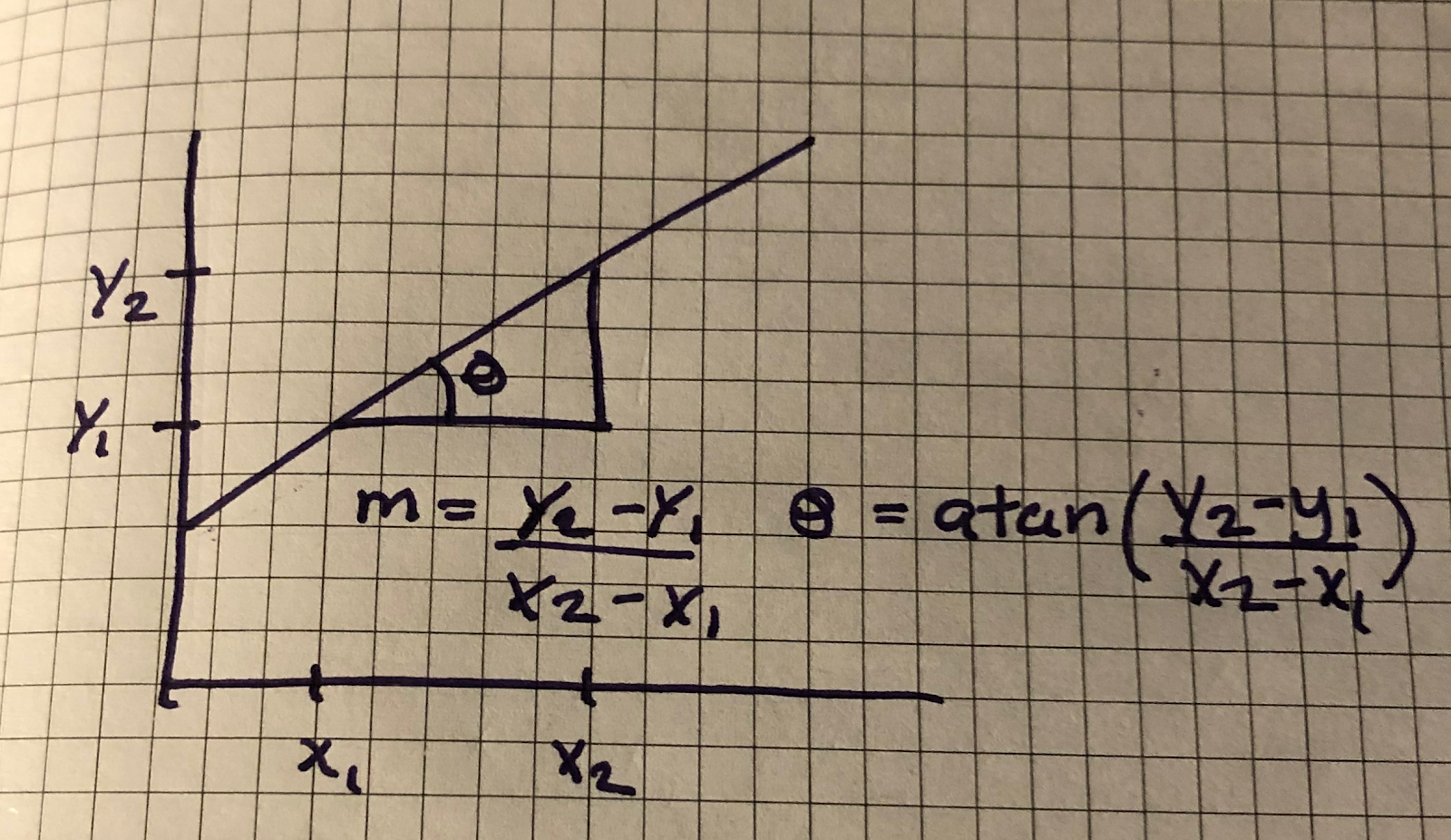
Recall from basic geometry, we can define this line as follows:

y = mx + b

where y is the height, b is y-intercept and m is our slope. Some simple algebra allows us to rearrange this equation to solve for the slope as follows:

m = (y – b) / x

Alternatively, we can find the slope from any two points on the line, p1 and p2, as follows:

m = (y2 – y1) / (x2 – x1) = dy / dx

This equation allows us to find a slope angle, 𝛳, given any two points:

𝛳 = atan(m)

Note, if our height value (y2 – y1) is big and our distance value (x2 – x1) is small, we get a large slope value (steep). Conversely, if our height value is small and our distance is big, we get a small slope value (flat). 

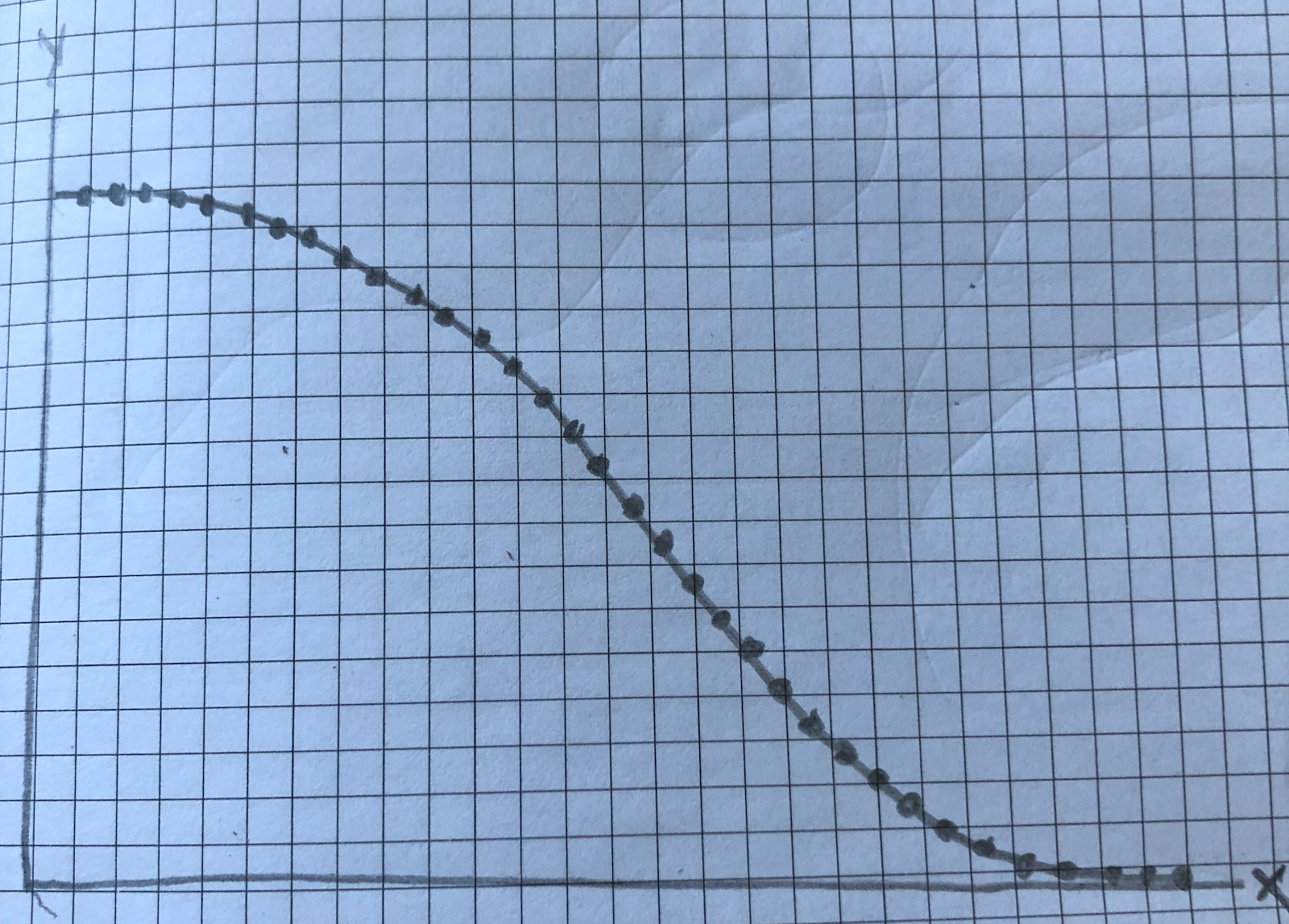
This works great for a line but what about curved terrain, like mountains? For any point on the curve, if we place a ski on it such that the ski touches the curve only once, we would find the tangent of the curve (the tangent represents the instantaneous slope at that point). The angle the ski makes with the horizon is the slope angle. 

With this in mind, we can now move the ski around adjusting it so that it touches the curve only once, giving us the slope at any point on the curve. If we moved the ski every meter or so along the curve and recorded the angle it makes with the horizon, we would get a pretty good picture of how the slope varies along the length of the curve (our terrain). We can achieve this by applying the equation above to solve for the slope using a series of discrete points as shown below:

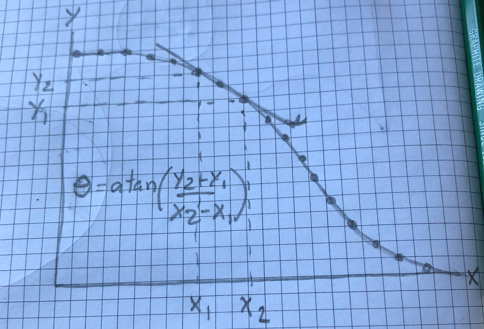
Now, it’s important to note here that the distance, x2 – x1, matters. If we choose an interval that is too big we might skip over a bunch of important information. On the other hand, if the distance is too small, we would end up spending the weekend calculating all the slopes and at some point the extra detail would do us little good. This could also result in a dataset that is just too large to take offline. 

Takeaway: Picking the right parameters for our slope angle calculation is critical for an accurate and portable representation of the terrain around us. 

So, this works fine for two dimensions, but we care about the real world and our world is three dimensional. Fortunately, we can extend this calculation to three dimensions as follows:

m = atan(sqrt(dy / dx ^ 2 + dy / dz ^ 2)) 

Again, all we’re really doing here is approximating the slope at a given point; and, if we have a good 3D representation of the earth’s surface, we can easily calculate slope angle anywhere on the planet. 

The Legend Matters

While this tool is incredibly powerful, it doesn’t substitute good decision-making. Slope angle visualization is just one tool in your toolbox, and like any tool, it is important that you learn how to use it safely. Slope angle visualizations can be misleading if we don’t understand the legend. For example, a slope angle color gradient not made for backcountry skiing might simply go from green to red, 0 to 90 degrees. While this is a perfectly accurate way to visualize slope, it doesn’t provide the best visualization for avalanche danger for recreationalists. We’ve chosen a gradient that we think intuitively highlights the danger zone for our users. In our Apps, green areas are 20-25 degrees—generally safer terrain. Yellow is 25-30 degrees, which is also generally safe. Once we start to approach the 30 degree mark, shown in red, in-field observation and careful terrain choice is recommended. 

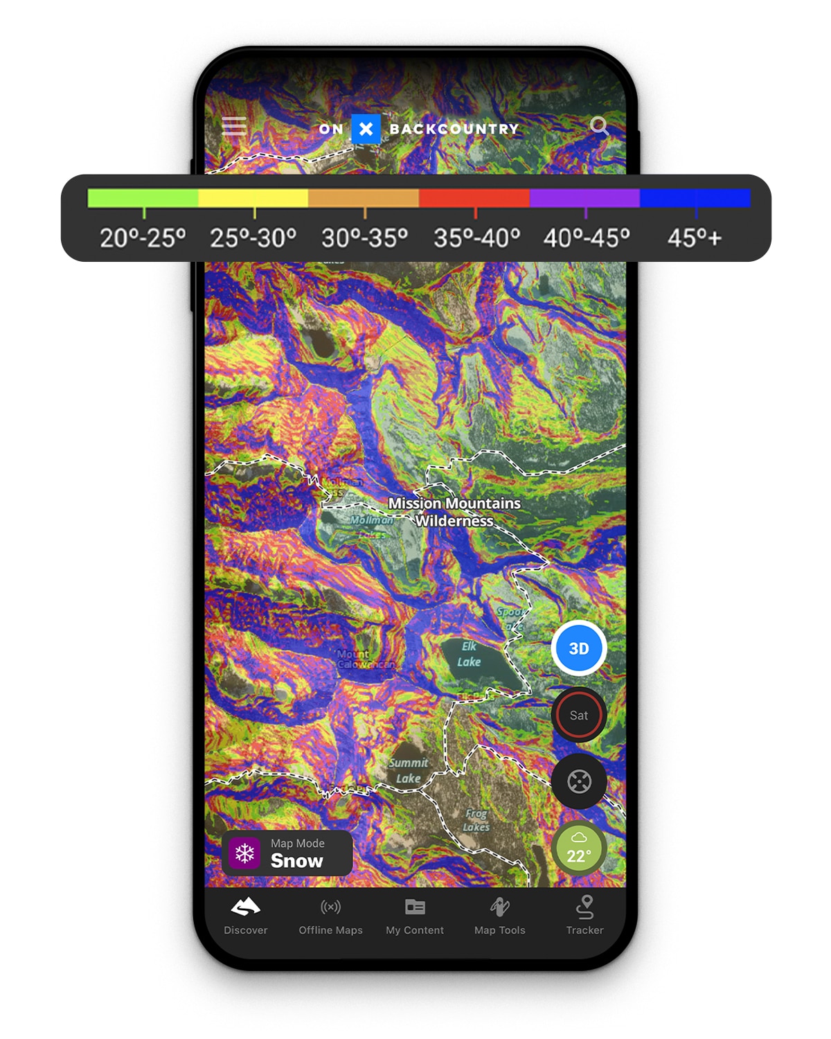
Takeaway: Slope angle visualization is a powerful tool but you must know how to use it properly. This starts by understanding exactly what the different colors indicate and what terrain lies above, around, and beneath you. 

Conclusion 

In this article we showed you how we calculate slope angle, where the data comes from, its accuracy, and how we’ve chosen to visualize it on the map. While onX has sourced the highest-resolution terrain data and double- (nay, triple-) checked our math to create this powerful tool for your adventure, Slope Angle is just one instrument in your arsenal to help you assess safety in the backcountry. As always, it is your responsibility to ensure that you are prepared for dangerous backcountry conditions, including checking avalanche and weather forecasts, knowing avalanche safety protocols, staying alert to changing conditions, and, of course, downloading Offline Maps.